The worm-like chain model is the most widely used model to describe polymers. Here are some notes about the derivation of the relationship between wlc model and the theory of elasticity.
elastic rod
Young's modulus
For a rod with a cross-section area \(A\) and length \(L\), when the deformation is small, the force follows the linear relation to the deforamtion, namely the to Hooke's law, \[ \begin{equation} F = k \Delta x \label{Hooke} \end{equation} \] If we consider the stress \(\sigma = \frac{F}{A}\) and the strain \(\epsilon = \frac{\Delta x}{L}\), then we can rewrite the above equation into, \[ \begin{equation*} \sigma = \frac{kL}{A} \epsilon = E \epsilon \end{equation*} \] where \(E = \frac{kL}{A}\) is the Young's modulus.
elastic bending
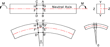
For a negative bending rod as shown below, the length of the neutral axis is the same with the rest length of the rod. So we can put the origin on the neutral axis and calculate the arc length \(H'G'\) at the distance \(y\) from the neutral axis.

So the strain of the infinitesimal arc \(H'G'\) is, \[ \begin{equation} \epsilon = - \frac{(R+y)\theta - R\theta}{R\theta} = - \frac{y}{R} \label{strain} \end{equation} \] where \(R\) is the radius of the curvature and \(\theta\) is the angle. Because it's negative bending, so \(R < 0\). But the minus sign in the above equation guarantees that the strain above the neutral axis is tensile and the strain below the neutral axis is compressive.
So we can easily get the stress, \[ \begin{equation} \sigma = E\epsilon = - E \frac{y}{R} \label{stress} \end{equation} \]
moment
Because the rod is under the static equilibrium, the external force and moment should be equal to the internal force and moment. Now we already know the stress \(\sigma\) in the cross section, so the momment is, \[ \begin{equation} M = - \int_{A} \sigma y dA = \frac{E}{R} \int_{A} y^2 dA \label{moment} \end{equation} \] The minus sign comes from the sign convention that negative bending rod has a negative bending moment. The moment of inertia \(I\) of the rectangular cross section is, \[ \begin{equation} I = \int_A y^2 dA = \frac{hw^3}{12} \label{inertia} \end{equation} \] where \(h\) and \(w\) are the height and the width of the rectangular cross section.
bending energy
From the Hooke's law, we know the internal energy is, \[ \begin{equation*} U = \int_{L}^{L+\Delta x} F dx = \int_{L}^{L+\Delta x} k x dx = \frac{1}{2} k \Delta x^2 \end{equation*} \] Let's say the area of cross section is \(A\) and the length of the rod is \(L\), \[ \begin{align*} U &= \int_{0}^{\epsilon} A \sigma L d\epsilon = AL \cdot \frac{1}{2} E \epsilon^2 \\ \partial{s} U &= \frac{1}{2} E \int_A \epsilon^2 dA \end{align*} \] Substituting \(\epsilon = -\frac{y}{R}\) into the above equation, we get the internal energy per unit length, \[ \begin{equation} \partial_{s}U = \frac{1}{2} \frac{EI}{R^2} = \frac{1}{2} EIc^2 \label{energy} \end{equation} \] The bending rigidity or bending stiffness is defined as \(\kappa = EI\).
If the rod has an intrinsic curvature \(c_0\), we can get the internal energy by Taylor expand the equation \(\eqref{energy}\) to 2nd-order, \[ \begin{equation*} U_{s}(c) = U_{s}(c_0) + \frac{1}{2} \kappa (c - c_0)^2 + O(c^3) \end{equation*} \] where the first term \(U_{s}(c_0) \ge 0\) is the bending energy at the rest bending curvature \(c_0\). The second term \(U_{s}'(c_0) = 0\) because the energy \(U_s\) is minimal at the position \(c_ 0\).
worm-like chain at surface
For a small bending, the curvature can be represented by \(c = \frac{\delta \theta}{\delta s}\), so the bending energy of an elastic rod with small length \(\delta s\) is quadratic in \(\delta \theta\). According to the Boltzmann distribution, the distribution of \(\delta \theta\) is hence Gaussian, \[ \begin{equation*} P(\delta \theta) = \exp(-\frac{1}{2} \frac{\kappa}{k_BT \delta s} \delta \theta^2) / Z \end{equation*} \] where \(Z = \int \exp(-\frac{1}{2} \frac{\kappa}{k_BT \delta s} \delta \theta^2) d\delta \theta\) is the partition function. Thus its Fourier transform is also Gaussian, \[ \begin{equation*} \widetilde{P}(\omega) = \exp(-\frac{1}{2} \frac{k_BT \delta s}{\kappa} \omega^2) \end{equation*} \] Because the angle deflection along the contour is additive, the distribution of the angle deflection at distance \(s\) is thus a convolution of many distributions of \(\delta s\), \[ \begin{equation} P(\theta) = \exp(-\frac{1}{2} \frac{\kappa}{k_BT s} \theta) / Z \label{dist} \end{equation} \] where \(s = \Sigma ~ \delta s\).
Let's say \(\boldsymbol{t}(s)\) is the unit tangent vector along the contour of the polymer chain. So we can use the tangent vector correlation function to describe the fluctuation extent of the polymer, \[ \begin{equation} <\boldsymbol{t}(0) \cdot \boldsymbol{t}(s)> = <\cos(\theta)> \label{corr} \end{equation} \] Here \(\cos(\theta)\) can be seen as the real part of \(\exp(-i \omega \theta)\) when \(\omega=1\), so the above correlation is equivalent to the Fourier trnasform, \[ \begin{equation} < \cos(\theta) > = \Big{(} \int \exp(-i \omega \theta) P(\theta) d\theta \Big{)}_{\omega=1} = \widetilde{P}(1) = \exp(- \frac{1}{2} \frac{k_BT}{\kappa} s) = \exp(- \frac{s}{2 l_p}) \label{decay} \end{equation} \] where the persistence length \(l_{p}\) is defined as \(\kappa / k_BT\).
polymers in 3D
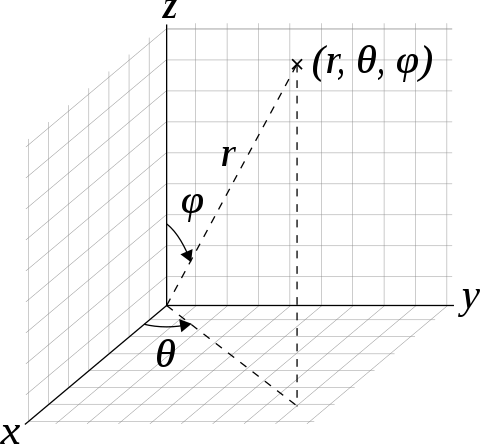
There are two transverse directions in 3D space which contribute to decorrelate the tangent vectors, i.e., if \(\boldsymbol{t}(0)\) is put along the x axis, the angle between two vectors \(\alpha\) is determined by two factors, \(\theta\) and \(\phi\). So the probability distribution of \(\alpha\) is the convolution of that of \(\theta\) and that of \(\phi\), \[ \begin{equation*} \widetilde{P}_{\alpha} = \widetilde{P}_{\theta} \widetilde{P}_{\phi} \end{equation*} \]

So the tangent correlation function in 3D space is, \[ \begin{equation*} < \cos(\alpha) > = \widetilde{P}_{\theta}(1) \widetilde{P}_{\phi}(1) \end{equation*} \] If the polymer is isotropic, then the tangent correlation decay would be doubled, \[ \begin{equation} < \cos(\alpha) > = \widetilde{P}(1)^2 = \exp(- \frac{s}{l_p}) \label{decay_3d} \end{equation} \]
Cauchy's exponential functional equation
One of properties of the tangent correlation function also implies that the exponential decay of correlation alone the contour. Considering two independent angles, \[ \begin{align*} < \cos(\theta + \phi) > &= \Big{(} \int \exp(-i\omega (\theta + \phi)) P(\theta+\phi) d(\theta+\phi) \Big{)}_{\omega=1} \\ &= \Big{(} \int \exp(-i\omega \theta) P(\theta) d\theta \int \exp(-i\omega \phi) P(\phi) d\phi \Big{)}_{\omega=1} \\ &= < \cos(\theta) > < \cos(\phi) > \end{align*} \] So it has the form of Cauchy's exponential functional equation, \[ \begin{equation*} f(x+y) = f(x)f(y) \end{equation*} \] The function which satifiies the above equatoin is an exponential function. We can Taylor expand it around \(x\), \[ \begin{equation*} f(x+y) = \sum_{n=0}^{\infty} \frac{1}{n!} f^{(n)}(x) y^n \end{equation*} \] Meanwhile, \[ \begin{equation*} f(x)f(y) = f(x) \sum_{n=0}^{\infty} \frac{1}{n!} f^{(n)}(0) y^n \end{equation*} \] So the coefficients before every \(y^n\) should be the same, \[ \begin{equation*} f^{(n)}(x) = f(x)f^{(n)}(0) \end{equation*} \] Let's set \(n=1\), \[ \begin{equation*} f'(x) = f(x) \cdot C \end{equation*} \] Then we get, \[ \begin{equation*} f(x) = A \exp(C x) \end{equation*} \]
Correlation of tangent vector
There is another way to get the relationship between \(l_p\) and \(\kappa\). If we Taylor expand both sides of the equation, \[ \begin{align*} \text{LHS} &= 1 - \frac{1}{2} < \delta \theta^2 > + O(\delta \theta^4) \\ \text{RHS} &= 1 - \frac{\delta s}{2L} + O(\delta s^2) \end{align*} \] So we have, \[ \begin{equation} < \delta \theta^2 > = \frac{\delta s}{l_p} \label{eq1} \end{equation} \]
According to statistic mechanics, we can calculate the correlation of bending angle from the energy, \[ \begin{align} <\delta \theta^2> &= \int \delta \theta^2 \exp(-U/k_BT) d\delta \theta \Big{/} \int \exp(-U/k_BT) d\delta \theta \\ &= \int \delta \theta^2 \exp(\delta s \cdot - \frac{1}{2} \frac{\kappa}{k_BT} (\frac{\delta \theta}{\delta s})^2) d\delta \theta \Big{/} \int \exp(\delta s \cdot - \frac{1}{2} \frac{\kappa}{k_BT} (\frac{\delta \theta}{\delta s})^2) d\delta \theta\\ &= \int \delta \theta^2 \exp(- \frac{1}{2} \frac{\kappa}{k_BT \delta s} \delta \theta^2) d\delta \theta \Big{/} \int \exp(- \frac{1}{2} \frac{\kappa}{k_BT \delta s} \delta \theta^2) d\delta \theta \label{secmom} \end{align} \] where the curvature \(c = \frac{\delta \theta}{\delta s}\). The numerator of \(\eqref{secmom}\) is the form of second moment of Gaussian distribution.
second moment of Gaussian distribution
For the integral, \[ \begin{equation*} I(s) = \int_{-\infty}^{\infty} \exp(-sx^2) dx = \sqrt{\frac{\pi}{s}} \end{equation*} \] Its partial derivative with respect to \(s\) is, \[ \begin{equation*} \partial_{s}I = - \int_{-\infty}^{\infty} x^2 \exp(-sx^2) dx = - \frac{\sqrt{\pi}}{2} s^{-\frac{3}{2}} \end{equation*} \] So we get the second moment of Gaussian distribution, \[ \begin{equation} M^{(2)} = - \partial_{s}I(1) = \frac{\sqrt{\pi}}{2} \label{secint} \end{equation} \]
persistence length and bending rigidity
Substituting equation \(\eqref{secint}\) into equation \(\eqref{secmom}\), \[ \begin{equation} < \delta \theta^2 > = (\frac{1}{2} \frac{\kappa}{k_BT \delta s})^{-\frac{3}{2}} \frac{\sqrt{\pi}}{2} \Big{/} (\frac{1}{2} \frac{\kappa}{k_BT \delta s})^{-\frac{1}{2}} \sqrt{\pi} = \frac{k_BT \delta s}{\kappa} \label{eq2} \end{equation} \]
Compared \(\eqref{eq1}\) and \(\eqref{eq2}\), we get, \[ \kappa = l_p k_BT \]
3D space
If polymers are in 3D space, on the one hand, the Taylor expansion is, \[ \begin{equation*} < \delta \alpha^2 > = \frac{2 \delta s}{l_p} \end{equation*} \] On the other hand, becuase the distribution of \(\alpha\) is a convolution of two Gaussian distributions, its variance would be doubled, \[ \begin{align*} < \delta \alpha^2 > &= \int \delta \alpha^2 P(\delta \alpha) d\delta \alpha \\ &= \int \delta \alpha_2 \exp(- \frac{1}{2} \frac{\kappa}{2 k_BT \delta s} \delta \alpha^2) d\delta \alpha \Big{/} Z \\ &= \frac{2 k_BT \delta s}{\kappa} \end{align*} \]
Eventually, it gives the same relationship between \(l_p\) and \(\kappa\) with that of 2D space.